Overview of Hamiltonian Monte Carlo
This portion of the recitation we prepared by Rosita Fu. It is an outline ofBetancourt’s paper. All figures and notation are from the paper. All lingering inaccuracies are my own.
This notebook will be presented in parallel with the next notebook by former TA Tom Röeschinger, which demonstrates the notion of a typical set alongside more detailed math/visualization and implementation of Hamiltonian Monte Carlo.
Notation
\(Q\): sample space constructed from parameter set (our priors!)
\(\pi\): target distribution
\(\pi(q)\): target density (this is our posterior!)
\(D\): D-dimensional sample space Q
Motivating interest:
Integrals that look like
If there is no analytical approach, we are left with numerical techniques. We essentially want to evaluate integrals by averaging over some representative region of parameter space instead of the entirety of parameter space. The problem is that the ordinary techniques do not handle high-dimensions very well. The expectation symbol is convenient notation, but the important thing to recognize here is that \(dq\) is some volume element and \(\pi(q)\) is our density at a given position \(q\).
Features of a high-dimensional space Q:
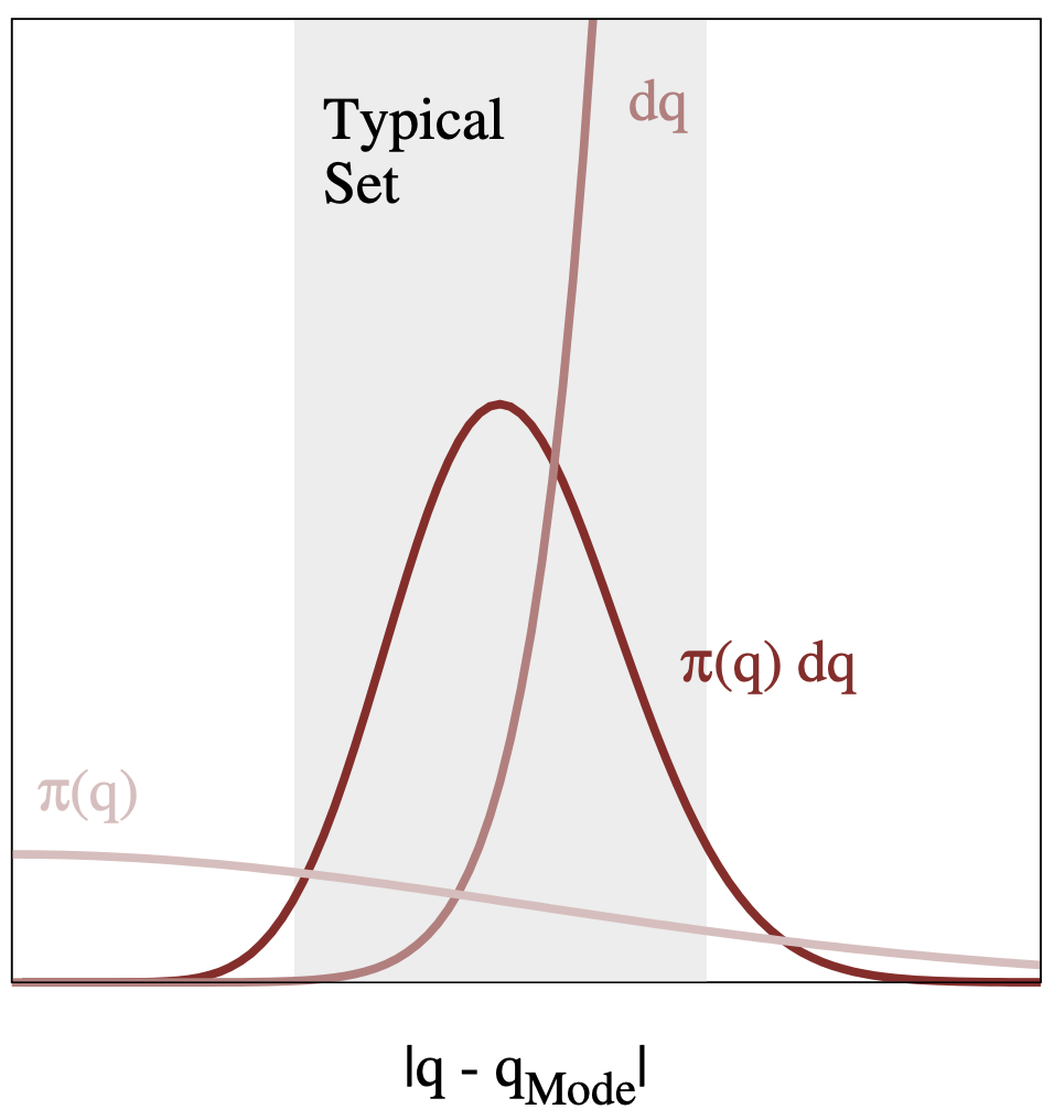
There is much more volume outside any given neighborhood than inside of it (consider simple case of partitioning 1D line, 2D box, 3D cube). We are thus interested in the neighborhoods in Q that balance both the denisty and volume in any given integration/expectation.
Volume and density end up pulling the mass to two different extremes—the result is that the predominant concentration of mass sits away from either extreme (high density: at the mode, concentrated in small volume blocks, high volume: mostly out in the tails, each “block” contributes small density, but there is an overwhelming number of blocks!)
This all motivates the definition of a typical set, the region of parameter space \(Q\) (volume) where most of our probability mass, the integrated quantity \(\pi(q) \mathrm{d}q\), sits.
But the question then remains: how do we design an algorithm to sample the typical set?
A helpful framework underpinning what we will try is a Markov chain. Loosely speaking, it’s a way to define the probability of a new element \(x_{i+1}\) that relies solely on the previous element \(x_{i}\) (hence a chain). Note that a Markov chain doesn’t specify how we transition to the next element, just that we do so solely on the basis of the previous one. One method is a transition matrix (like Metropolis-Hastings), but you could imagine many ways to creatively structure a new transition (which we will see w/ the Hamiltonian). The particular features of Markov chains we will take advantage of:recurrenceandergodicity. small note: “Monte Carlo” basically alludes to anything stochastic (as opposed to deterministic) whereas Markov Chain defines this type of sampling/walking motion… note that these are the “chains” we refer to!
A recurrent and ergodic markov chain tells us that given infinite time, samples from a random walk dictated by a given transition matrix will eventually be equivalent to a sample from the target distribution itself. This directly gives us samples from the typical set. This is precisely what we are trying to do!!… except on finite time. This is a type of central limit theorem, where
\[f_N^{\mathrm{MCMC}} \sim \mathcal{N} (\mathbb{E}_{\pi}[f], \mathrm{SE}_\mathrm{MCMC})\]This finite limitation means we need to define some performance metrics to evaluate our chains.
ESS: The effective sample size tells us the effective number of exact samples “contained” in the Markov chain (think correlation btw samples).
\(\hat{r}\): evaluates ergodicity by looking at variance between and within chains,
\[\hat{r} = \sqrt{1+B/W}\]we particularly want the ratio \(B/W\) to be small, and \(\hat{r} < 1.01\)
Divergences: Markov chains have a habit of “skipping over” regions of high curvature. To deal with this, some algorithms implement ways for the chain to hover near the pathological region, but this overcompensates and leads to oscillating estimators. Note: these above metrics apply to all Markov chains, though they may differ in their computation/usage. They are descriptions of the diffusivity properties of any finite “chain” we could ask our computer to make.
One Markov transition you have explored in set 4 was the Metropolis-Hastings. Though the Metropolis Hastings algorithm is incredibly useful in low-dimensionality, it struggles irredeemably in higher dimensions (think funnels and high curvature!) Think about why this is. If you have an exponentially-increasing number of directions to “turn”, and the adjacent elements of the target set are in a singular direction, you will keep rejecting steps and your random walker will be incapacitated… We can try pushing a larger acceptance probability, but the small jumps lead to an incredibly sluggish chain!
One thing we have not utilized is the actual geometry of the target probability density \(\pi(q)\). What we intuitively want is some vector field that incrementally points along the typical set, an overall trajectory. The first vector field you might think of is the gradient… but this just pushes us back to the mode! A vector field assigns a vector (direction + magnitude) at every point in parameter space Q. A gradient is an operator that takes in some point (\(q_1, q_2, q_3\)) and returns (\(\partial{f}/\partial{q_1}\), \(\partial{f}/\partial{q_2}\), \(\partial{f}/\partial{q_3}\)); i.e. it is a directional derivative.
So this all leads us to … 🎉 Hamiltonian Monte Carlo! 🎉
Now that the objective is clear, we will construct and explore mathematical objects we intuit might be useful to the problem at hand, specifically re-casting a problem of geometry to one of classical physics. This hearkens back to one of the most satisfying features of probability: every probabilistic system has a mathematically equivalent physical system.
Here are the objects in the metaphor to come:
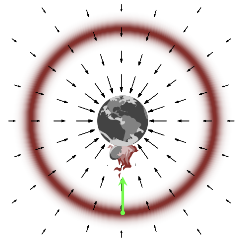
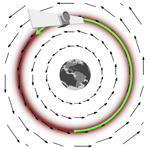
mode: planet
gradient: gravitational field
typical set: orbit trajectory
samples: satellite trajectory
The task of finding a typical set then translates to the objective of placing a satellite in a stable orbit around the planet. Intuitively, a stable orbit conserves energy, otherwise we either crash into the planet (being pulled towards the mode of our target distribution/heavily biased by the density), or eject out into space (running away from the mode and the typical set, biased by the volume).
To do so, we intuit that we need to introduce some auxiliary momentum parameters (denote with \(p\)). This doubles our parameter space from D to 2xD-dimensional space; together with our target parameter space, we call this the phase space.
We now expand our target distribution to include the momentum dimensions, and construct a joint probability distribution over phase space, we call this the canonical distribution:
Note that if we marginalize out momentum :math:`p`, we recover :math:`pi(q)`. This means that exploring the typical set in phase space :math:`pi(q,p)` is equivalent to exploring the typical set of the target distribution :math:`pi(q)`
We can then write the canonical distribution in terms of a Hamiltonian function \(H(q,p)\) with a kinetic and potential energy:
:nbsphinx-math:`begin{align}\ pi(q, p) &= pi(p | q) pi(q) := e^{-H(q, p)} \[0.8em] H(q, p) &= -log pi(q, p) \[0.5em]
&= -log pi(p | q) - log pi(q) \[0.5em] &= K(p, q) + V(q)\[0.8em]
end{align}`
\begin{align} \boxed{ K(p, q) = -\log \pi(p | q) \\[0.5em] \hspace{0.9em} V(q) = - \log \pi(q) } \end{align}
We call the total “energy” the actual value of the Hamiltonian. Note that our energy terms \(K\) and \(V\) are in units of log-pdf’s! The conservation of energy thus could be interepreted as some conservation of being “lifted” up into phase space.
\begin{align} E &= H(q, p) \\[0.5em] &= -\log \pi(q, p) \\[0.5em] &= K+V \end{align}
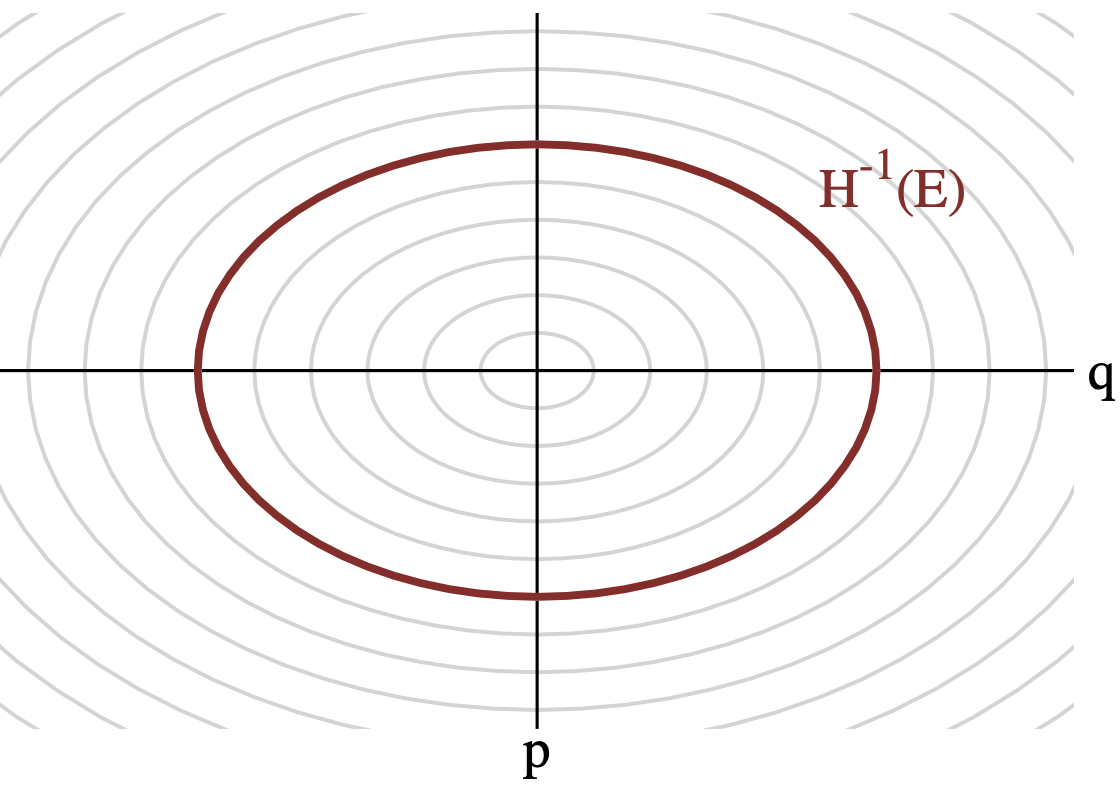
Thus, every point in (q, p) has some associated energy, and for a given energy \(E\), there exists a level set \(\Omega\) in \((q, p)\) that have the same energy. Multiple energies give us concentric circles (think contour maps) in \((q, p)\), and it is possible to reparametrize \((q, p)\) as \((E, \Omega_E)\), where \(\Omega_E\) is the position within the level set. With the re-parametrization, we then have:
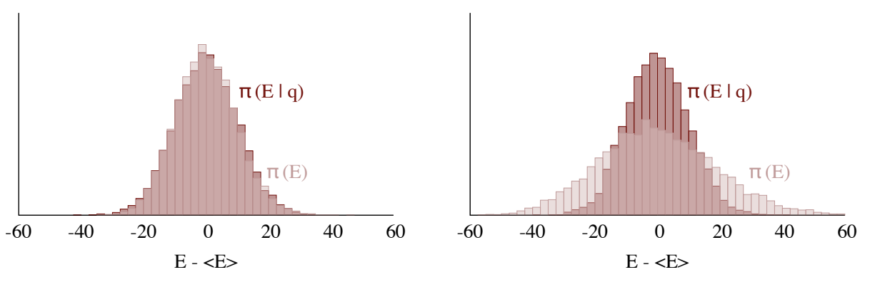
where \(\pi(E)\) is the marginal energy distribution, and \(\pi(\Omega_E | E)\) the microcanonical distribution. You can easily visualize \(\pi(E)\) as a distribution over the rings you see below.
Now that we have all this math set-up, let’s see what we can actually do with it!
The Ideal Hamiltonian Markov Transition
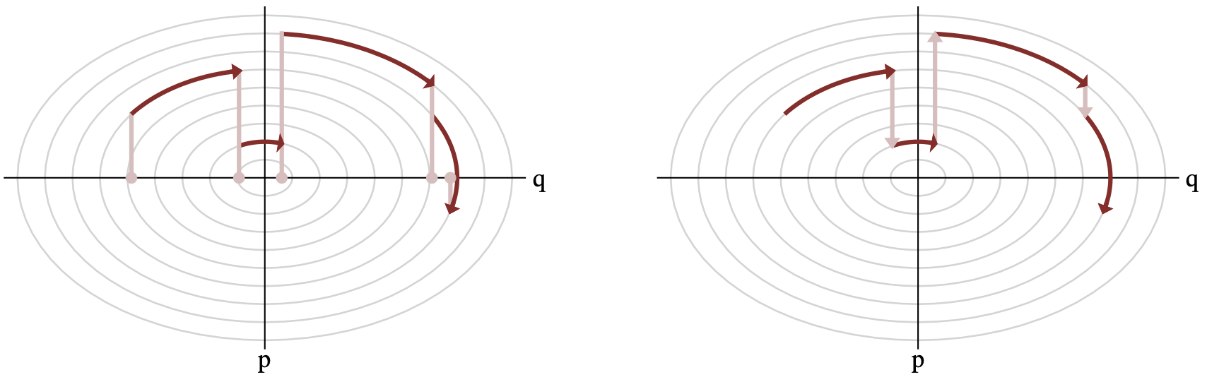
Referring to the boxed equation above, note that our potential energy is completely characterized by our target distribution \(\pi(q)\), whereas the kinetic energy must be specified. Specifying \(K\) would allow us to sample a point in phase space given an initial point in \(q\):
Once we have some \(p\) given \(q\), we have \((q, p)\); we can then explore the jointly typical set by integrating Hamilton’s equations for some time to get a trajectory \(\phi(q, p)\)
\begin{align} \cfrac{\mathrm{d}q}{\mathrm{d}t} &= + \cfrac{\partial{H}}{\partial{p}} = \cfrac{\partial{K}}{\partial{p}} \\[0.2em] \cfrac{\mathrm{d}p}{\mathrm{d}t} &= - \cfrac{\partial{H}}{\partial{q}} = -\cfrac{\partial{K}}{\partial{q}} - \cfrac{\partial{V}}{\partial{q}} \\[0.3em] \end{align}
Given that marginalizing out p recovers \(\pi(q)\), we can simply ignore the momentum and return to the target parameter space \(q\):
Altogether, this is what four transitions looks like:

Let’s pause for a moment. What have we actually done here?
We started off with some intuition about momentum, and introduced the concept of a phase space. This doubled our dimension—so every \(q_i\) dimension now has some associated momentum \(p_i\). So where/why did the Hamiltonian come in?
We essentially needed to somehow expand our probability space over our momentum dimensions, and the very definition that unlocked this for us was the following:
The exponent leads to a logarithm that then turns our product into a sum K + V (each term a log-probability density). This sum meant we could decouple the process into a stochastic step and a deterministic step.
Stochastic step: lifting \(q\) into \((q, p)\) by defining some distribution \(K = -\log(p|q)\)
Deterministic step: integrating Hamilton’s equations of motion for \((q, p)\) over time to get some trajectory \(\phi_t(q, p)\); we then take the last position of this integration, and retrieve \(q\)… this becomes the next iteration of our Markov chain!
Repeatedly doing ^ those two steps gives us a Hamiltonian Monte Carlo MarkovChain. Does it make sense what it means to initialize 4 chains in Stan, and how each one is transitioning?
The deterministic step explores individual energy level sets, while the stochastic step explores between level sets. Both steps require some tuning on the user-end, or at least looking at some diagnostics.
Note: What does this have to do with the typical set? Out in the tails of the target distribution, momentum sampling and projection allows the chain to rapidly fall in toward the typical set. Once inside the typical set, trajectories \(\phi_t(q, p)\) move swiftly through phase space and remain constrained to the typical set.
Actual Implementation of Hamiltonian Markov Transition Considerations
Here’s an overview of what remains to be done: - (A) Choose \(K\) to sample momentum \(p\) (stochastic step). - Euclidean-Gaussian - Riemannian-Gaussian - E-BFMI
Integration method (deterministic step)
💚 Symplectic integration 💚 does not drift…
regions of high curvature?
Integration time (deterministic step)
vary integration time dynamically
heavier-tailed posterior → longer integration time
(A) Optimizing Choice of Kinetic Energy \(K(q, p)\)
We effectively need to choose some conditional probability distribution for the momentum. Ideally, the choice would ensure that the energy level sets are as uniform as possible, which means we’d be able to explore the breadth of \(\log\pi(q, p)\) extremely efficiently.
As \(K\) can be any function, we have infinite options, but Euclidean-Gaussian and Riemannian-Gaussian are the current standards that have performed quite well.
The next notebook goes into the math in a bit more detail, but for now we will state the definitions and their motivations:
Euclidean-Gaussian Kinetic Energies:
Riemannian-Gaussian Kinetic Energies:
Motivation: We want to choose a kinetic energy such that the microcanonical distribution \(\pi(E|q)\) looks like the marginal energy distribution\(\pi(E)\) (left). Otherwise, our chain may not be able to completely explore the tails of the target distribution (right).
E-BFMI: Stan is already doing the work of choosing \(K\) and tuning it; on the user end, we see the E-BFMI diagnostic that tells us how Stan’s algorithms are doing on this front.
The empirical Bayesian fraction of missing information identifies when the momentum resampling is inefficiently exploring the energy level sets, and is essentially the ratio:
Do you see how the ratio relates to the above plots, and how we don’t want lower E_BFMI’s? Generally, E-BFMI < 0.3 have proven problematic.
Intuition for Gaussian KE: Note that despite a complicated covariance matrix, our final choice for the conditional distribution \(K\) is a multivariate Gaussian with a pretty involved-covariance matrix. It may seem arbitrary to pick a Gaussian, but a possible reason it has performed so well is that in higher dimensional models, we can think of \(\pi(E)\) as a convolution of more and more parameters, and under relatively weak conditions, follows a central limit theorem.
Now, what is \(M\)?? We want \(M^{-1}\) to closely resemble the covariance of the target distribtuion to de-correlate the target distribuion, and make energy level sets that are more and more uniform and easier to explore. In practice, the empirical estimate for the target covariance is calculated from the Markov chain itself in an extended warm-up phase$
(B) Integration method
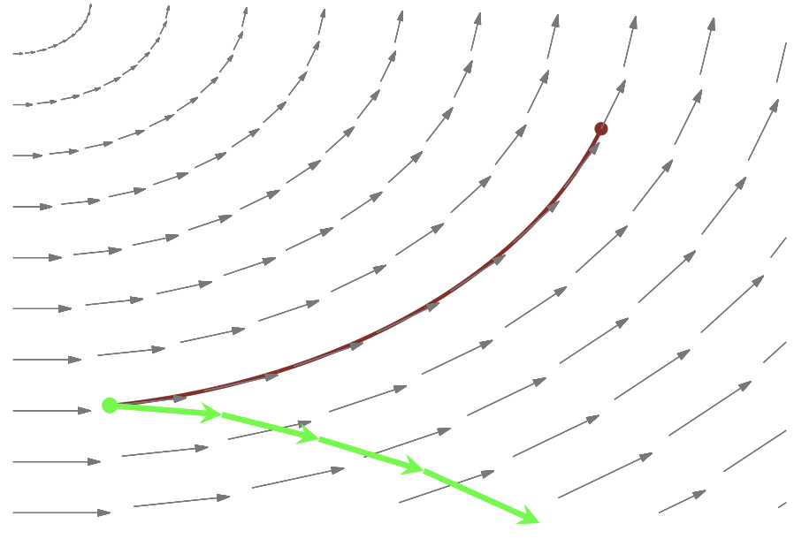
After being lifted to \((q, p)\), we need to integrate! Unfortunately, there is no closed-form solution to Hamilton’s equations, so we must resort to numerical methods. - Though there are many ODE-solvers out there, most suffer from drift as we integrate longer and longer trajectories, and the errors additively push our integrated trajectory away from the exact trajectory.
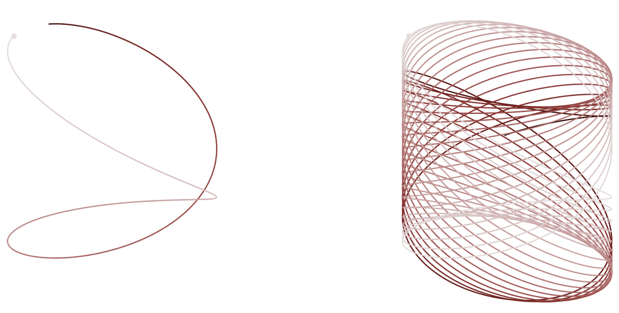
Symplectic integrators are a family of numerical solvers that are robust to drift; they have the special property of preserving phase space volume! Their errors lead to trajectories that oscillate around the exact level set, even as we integrate for longer and longer times.
 \(\hspace{3em}\)
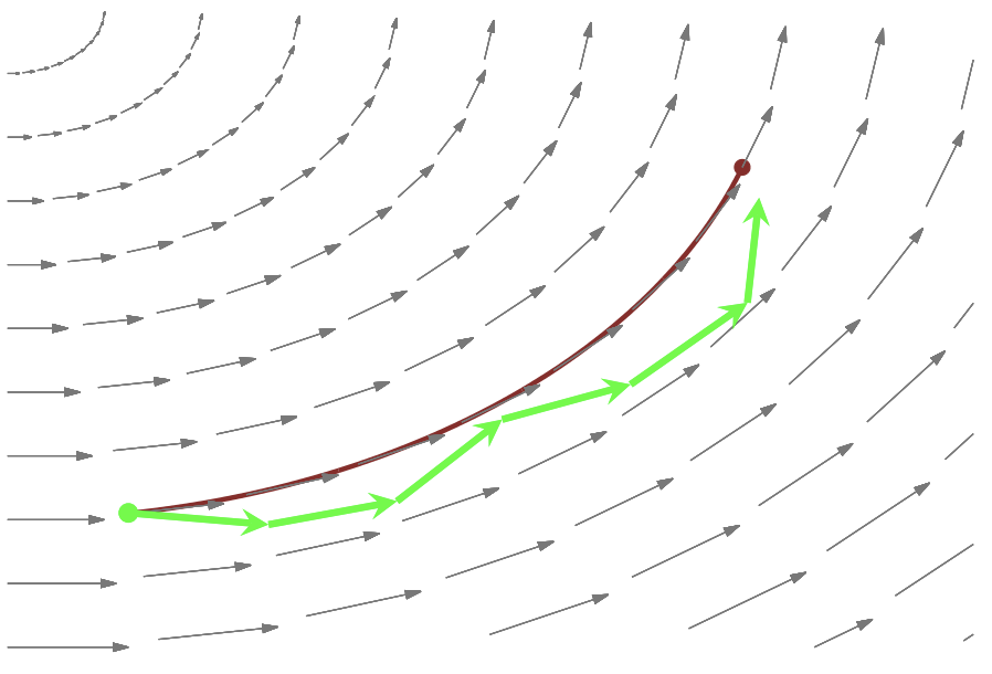
Note: this is where the leapfrog integrator is used, given some time discretization step size \(\epsilon\).
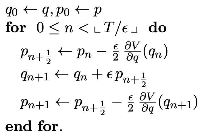
However; even symplectic integrator suffers from regions of high curvature; this induces a divergence. - From a modeling perspective, one approach to eliminate divergences is noncentering. This greatly smoothens out regions of high curvature. - From a tuning perspective, we can try decreasing the step size :math:`epsilon` by increasing ``adapt_delta``. If divergences persist regardless of how small the step size, this calls for stronger priors or an alternative representation of the model. - Use the divergences diagnostically; their existence should prompt suspicion, as the estimators (as is) will be biased.
(C) Integration time
Now that we have the method, we need to know just how long to integrate for each transition.
Integration time aims to explore “just enough” of each level set. But how do we quantify this idea on computational time scales?
Here’s a simple thought experiment: Think of a posterior \(\pi_\beta(q)\) of below form, where \(\beta\) describes how heavy our posterior tail is. With a Euclidean-Gaussian KE (denoted \(\mathcal{N}\)), the optimal integration time \(T_{\mathrm{optimal}}\) scales with the energy of the level set \(H(q,p)\) containing the trajectory:
\begin{align} \pi_\beta (q) &\propto e^-{|q|}^\beta \\[0.2em] \pi(p | q) &= \mathcal{N}(0,1)\\[0.2em] T_{\mathrm{optimal}} (q|p) &\propto [H(q,p)]^{\frac{2-\beta}{2 \beta}} \end{align}
The insight here is that as \(\beta < 2\), the target distribtion becomes heavier, and the optimal integration time grows with E as we try to explore the tails. This motivates the algorithmic design to dynamically vary the integration time; Stan uses a modified No-U-Turn termination criteria to know when to stop, by evaluating forward and backward trajectories.
Concluding thoughts
Hopefully what Stan is doing under-the-hood is less mysterious to you now (although so much more impressive!) It really is trying to accomplish something much more robust than what came before. The main takeaway perhaps begins with that of the typical set, and how life changes in higher dimensions. Once the objective is clear, a very clean theoretical framework—the Hamiltonian—exploits the geometry of the typical set itself to glean insight into integrals and distributions otherwise much too complex to solve. In implementation and usage, the pathologies we might face motivates principled strategies and approaches to modeling.