Probability as the logic of science
We thought about the process of scientific inquiry last term, but we visit it again here to refresh us about where statistical inference fits in the process of doing science. In the figure below, we have a sketch of the scientific processes. This cycle repeats itself as we explore nature and learn more. In the boxes are milestones, and along the arrows in orange text are the tasks that get us to these milestones.
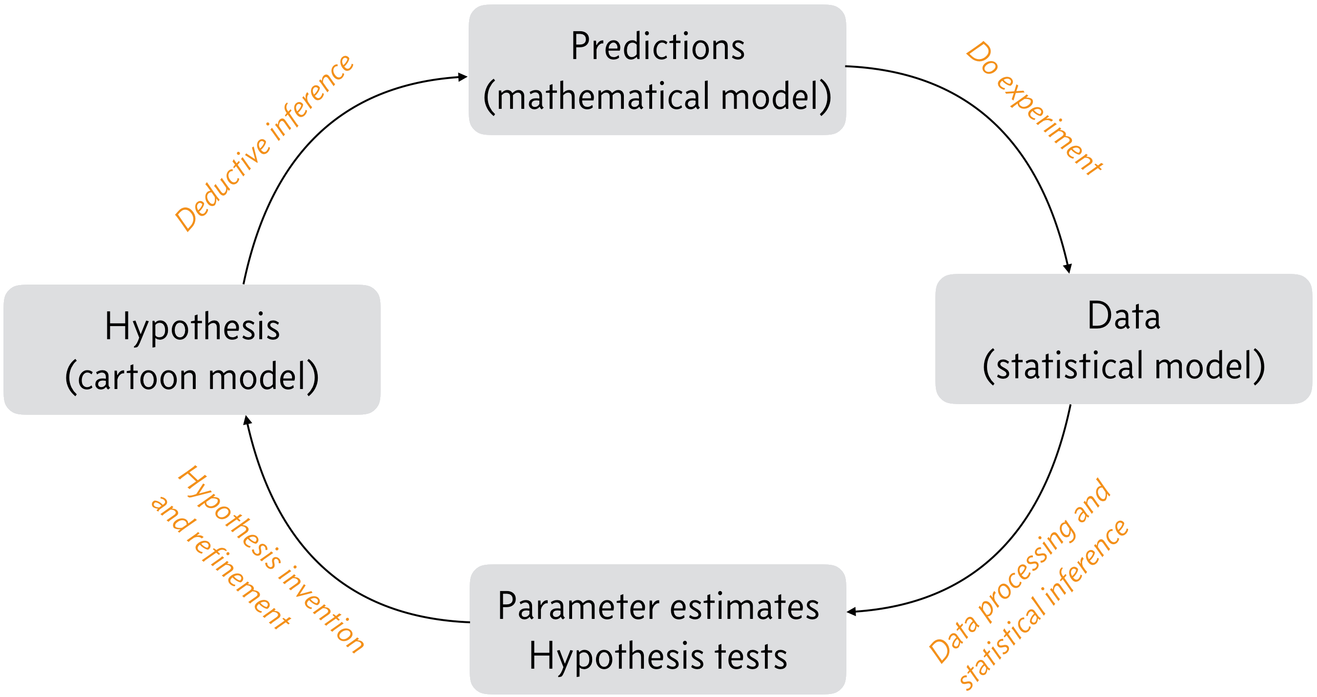
A sketch of the scientific process. Adapted from Fig. 1.1 of P. Gregory, Bayesian Logical Data Analysis for the Physical Sciences, Cambridge, 2005.
Let’s consider the tasks and their milestones. We start in the lower left.
Hypothesis invention/refinement. In this stage of the scientific process, the researcher(s) think about nature, all that they have learned, including from their experiments, and formulate hypotheses or theories they can pursue with experiments. This step requires innovation, and sometimes genius (e.g., general relativity).
Deductive inference. Given the hypothesis, the researchers deduce what must be true if the hypothesis is true. The result of deductive inference is a set of (preferably quantitative) predictions that can be tested experimentally. You have done a lot of this in your study to this point, e.g., given X and Y, derive Z. Logically, this requires a series of strong syllogisms:
If A is true, then B is true.
A is true.
Therefore B is true.
Do experiment. This requires work, and also its own kind of innovation. Specifically, you need to think carefully about how to construct your experiment to test the hypothesis. It also usually requires money. The result of doing experiments is data.
Statistical (plausible) inference. This step is perhaps the least familiar to you, but this is the step that this course is all about. I will talk about what statistical inference is next; it’s too involved for this bullet point. But the result of statistical inference is knowledge about how plausible a hypothesis and estimates of parameters under that hypothesis are.
What is statistical inference?
As we designed our experiment under our hypothesis, we used deductive logic to say, “If A is true, then B is true,”” where A is our hypothesis and B is an experimental observation. This was deductive inference.
Now, let’s say we observe B. Does this make A true? Not necessarily. But it does make A more plausible. This is called a weak syllogism. As an example, consider the following hypothesis/observation pair.
A = Wastewater injection after hydraulic fracturing, known as fracking, can lead to greater occurrence of earthquakes.
B = The frequency of earthquakes in Oklahoma has increased 100 fold since 2010, when fracking became common practice there.
Because B was observed, A is more plausible. A is not necessarily true, but definitely more plausible.
Statistical inference is the business of quantifying how much more plausible A is after obeserving B. In order to do statistical inference, we need a way to quantify plausibility. Probability serves this role.
So, statistical inference requires a probability theory. Thus, probability theory is a generalization of logic. Due to this logical connection and its crucial role in science, E. T. Jaynes said that probability is the “logic of science.”
The problem of probability
We know what we need, a theory called probability to quantify plausibility. We more formally [1] defined probably last term. We will not formally define probability here, but use our common sense reasoning of it. Nonetheless, it is important to understand that there are two dominant interpretations of probability.
Frequentist probability.
In the frequentist interpretation of probability, the probability \(P(A)\) represents a long-run frequency over a large number of identical repetitions of an experiment. These repetitions can be, and often are, hypothetical. The event \(A\) is restricted to propositions about random variables, a quantity that can very meaningfully from experiment to experiment. [2]
Bayesian probability.
Here, \(P(A)\) is interpreted to directly represent the degree of belief, or plausibility, about \(A\). So, \(A\) can be any logical proposition.
You may have heard about a split, or even a fight, between people who use Bayesian and frequentist interpretations of probability applied to statistical inference. There is no need for a fight. The two ways of approaching statistical inference differ in their interpretation of probability, the tool we use to quantify plausibility. Both are valid. In fact, we used frequentist methods exclusively last term to great effect.
In my opinion, the Bayesian interpretation of probability is more intuitive to apply to scientific inference. It always starts with a simple probabilistic expression and proceeds to quantify plausibility. It is conceptually cleaner to me, since we can talk about plausibility of anything, including parameter values. In other words, Bayesian probability serves to quantify our own knowledge, or degree of certainty, about a hypothesis or parameter value. Conversely, in frequentist statistical inference, the parameter values are fixed, and we can only study how repeated experiments will convert the real parameter value to an observed real number.
Going forward, we will use the Bayesian interpretation of probability.
Desiderata for Bayesian probability
In 1946, R. Cox laid out a pair of rules based on some desired properties of probability as a quantifier of plausibility. These ideas were expanded on by E. T. Jaynes in the 1970s. The desiderata are
Probability is represented by real numbers.
Probability must agree with rationality. As more information is supplied, probability must rise in a continuous, monotonic manner. The deductive limit must be obtained where appropriate.
Probability must be consistent.
Structure consistency: If a result is reasoned in more than one way, we should get the same result.
Propriety: All relevant information must be considered.
Jaynes consistency: Equivalent states of knowledge must be represented by equivalent probability.
Based on these desiderata, we can work out important results that a probability function must satisfy. I pause to note that one can generally define probability without a specific interpretation in mind, and it is valid for both Bayesian and frequentist interpretations, and we did this last term.
Two results of these desiderata (worked out in chapter 2 of Gregory’s book) are the sum rule and the product rule.
The sum rule, the product rule, and conditional probability
The sum rule says that the probability of all events must add to unity. Let \(A^c\) be all events except \(A\), called the complement of \(A\). Then, the sum rule states that
Now, let’s say that we are interested in event \(A\) happening given that event \(B\) happened. So, \(A\) is conditional on \(B\). We denote this conditional probability as \({P(A\mid B)}\). Given this notion of conditional probability, we can write the sum rule as
for any \(B\).
The product rule states that
where \(P(A,B)\) is the probability of both \(A\) and \(B\) happening. The product rule is also referred to as the definition of conditional probability. It can similarly be expanded as we did with the sum rule.
for any \(C\).
Application to scientific measurement
This is all a bit abstract. Let’s bring it into the realm of scientific experiment. We’ll assign meanings to these things we have been calling \(A\), \(B\), and \(C\).
So, we may be interested in the probability of obtaining a data set \(y\) given some set of parameters \(\theta\) . In other words, we want to learn about \(P(y|\theta)\).
To go a bit further, let’s rewrite the product rule.
We have explicitly written all other information we know going into the experiment as \(I\). This is always present, so henceforth we will not write it, but we should keep in mind that we are not doing science in a vacuum; \(I\) is always there.
Ahoy! The quantity \(P(\theta \mid y)\) is exactly what we want from our statistical inference. This is the probability for values of a parameter, given measured data.
But wait a minute. The parameter \(\theta\) is not something that can vary meaningfully from experiment to experiment; it is not a random variable. So, in the frequentist picture, we cannot assign a probability to it. That is, \(P(\theta\mid y)\) and \(P(y, \theta)\) do not make any sense. So, in the frequentist perspective, we can really only analyze \(P(y\mid \theta)\). But in a Bayesian perspective, we can analyze what we want, \(P(\theta\mid y)\)!
Now, how do we compute it \(P(\theta\mid y)\)?
Bayes’s Theorem
Note that because “and” is commutative, \(P(\theta, y) = P(y, \theta)\). So, we apply the product rule to both sides of the seemingly trivial equality.
If we take the terms at the beginning and end of this equality and rearrange, we get
This result is called Bayes’s theorem. This is far more instructive in terms of how to compute our goal, which is the left hand side. The quantities on the right hand side all have meaning. We will talk about the meaning of each term in turn, and this is easier to do using their names; each item in Bayes’s theorem has a name.
The prior probability.
First, consider the prior, \(P(\theta)\). As probability is a measure of plausibility, or how believable a hypothesis is. This represents the plausibility about hypothesis \(\theta\) given everything we know before we did the experiment to get the data.
The likelihood.
The likelihood, \(P(y\mid \theta)\), describes how likely it is to acquire the observed data, given the hypothesis or parameter value \(\theta\). It also contains information about what we expect from the data, given our measurement method. Is there noise in the instruments we are using? How do we model that noise? These are contained in the likelihood.
The evidence.
I will not talk much about this here, except to say that the evidence, \(P(y)\) can be computed from the likelihood and prior, and is also called the marginal likelihood, a name whose meaning will become clear in the next section. [3]
The posterior probability.
This is what we are after, \(P(\theta\mid y)\). How plausible is the hypothesis or parameter value, given that we have measured some new data? It is calculated directly from the likelihood and prior (since the evidence is also computed from them). Computing the posterior distribution constitutes the bulk of our inference tasks.