Homework 9.2: Inferring fitness from pooled competition assays (100 pts)
This problem is based onRazo-Mejia, Mani, and Petrov, Bayesian inference of relative fitness on high-throughput pooled competition assays, Plos Computational Biology, in press. Manuel Razo-Mejia provided valuable consultation.
A pooled competition assay works as follows. A population of cells of different strains are placed in minimal media and are allowed to grow for a given time interval. The cells are then diluted and placed in a fresh solution of minimal media. This is repeated several times.
Most of the cells that are in the initial sample are an unlabeled reference strain. Each of the other strains has a unique barcode sequence integrated into its genome. Among these other strains a neutral lineages, which have barcodes but are otherwise equivalent to the reference strain. Immediately prior to each dilution, some volume of cells are collected and sequencing is done to get counts of cells via counts of the respective barcodes. The schematic below, taken from the Razo-Mejia, Mani, and Petrov paper illustrates this process.
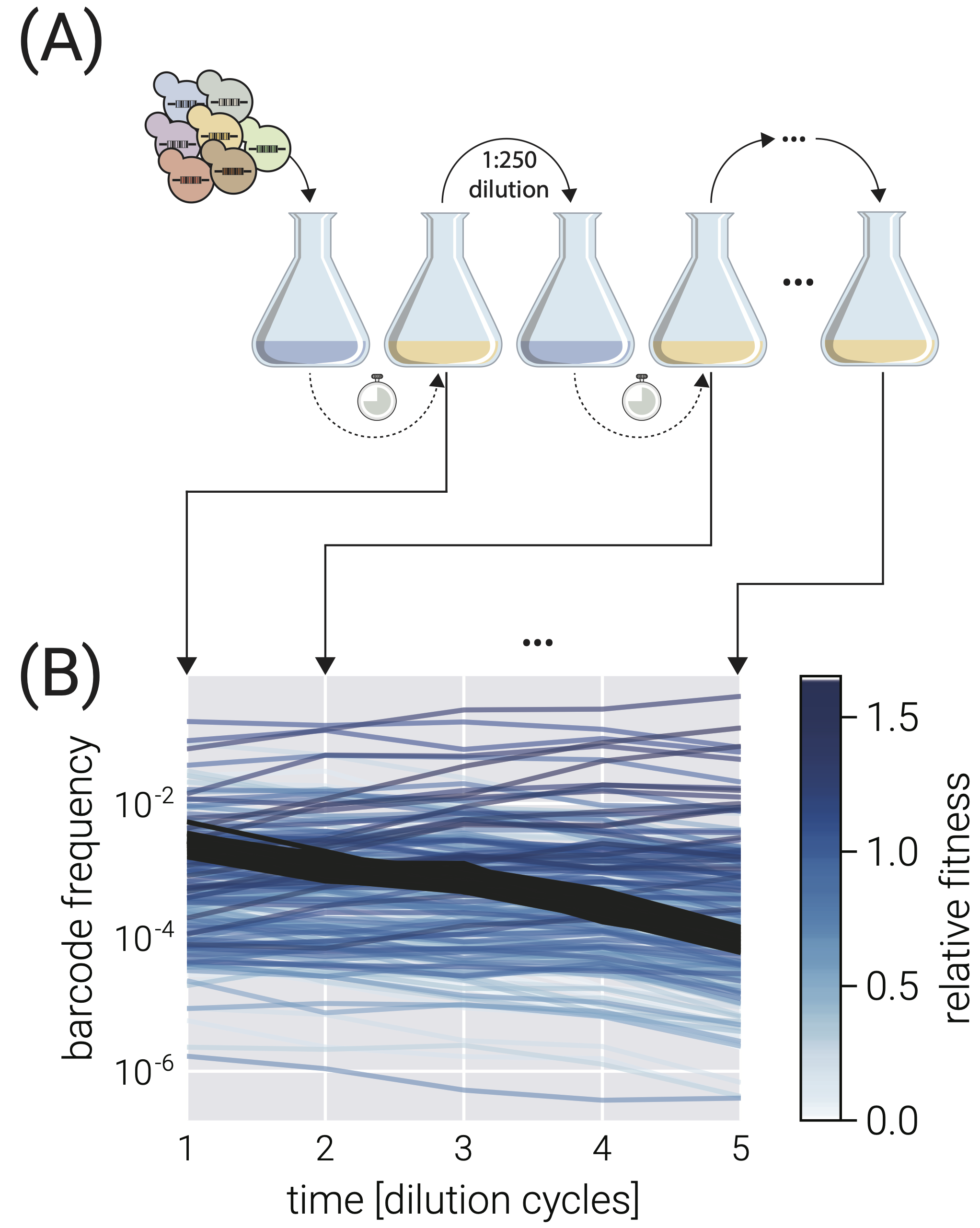
In the above plot, the black lines are the neutral strains, whose barcode frequency decreases over time, being outcompeted by some of the other non-neutral strains.
So, the output of the experiment is a set of read counts for each barcode at each discrete time point. Let us now develop a model connecting these read counts of barcodes to fitness of the strains of cells that have the respective barcodes. We follow the treatment in the Razo-Mejia paper.
a) Let \(r_t^{(b)}\) be the number of reads of barcode \(b\) at the end of cycle number \(t\). This is what the data set consists of. In our model, we will will model \(r_t^{(b)}\) as being Poisson distributed. Specifically,
\begin{align} r_t^{(b)} \sim \text{Pois}(\lambda_t^{(b)})\;\; \text{ for each } t, b. \end{align}
Why is this a reasonable model?
b) Let \(f_t^{(b)}\) be the frequency of barcode \(b\) in the culture at the end of cycle number \(t\). The frequency is defined as the relative abundance of a certain strain at a given point in time. This can be computed from the inferred Poisson rate parameters as
\begin{align} f_t^{(b)} = \frac{\lambda_t^{(b)}}{\sum_b \lambda_t^{(b)}}. \end{align}
The fundamental assumption in the above equation is that the read count for a given barcode is proportional to the number of cells possessing the barcode.
Through high-resolution lineage tracking experiments (see citations in the Razo-Mejia paper), we know phenomenologically that frequency of a given barcode grows or decays exponentially, such that
\begin{align} f_{t+1}^{(b)} = f_t^{(b)}\,\mathrm{e}^{s^{(b)} - \bar{s}_t}, \end{align}
where \(s^{(b)}\) is referred to as the relative fitness, that is the fitness relative to the reference strain. The parameter \(\bar{s}_t\) is the mean fitness of the entire culture at the end of cycle number \(t\). The above equation is typically written as
\begin{align} \ln \gamma_{t+1}^{(b)} = s^{(b)} - \bar{s}_t, \end{align}
where
\begin{align} \gamma_{t+1}^{(b)} = \frac{f_{t+1}^{(b)}}{f_t^{(b)}}. \end{align}
The value of the relative fitness \(s^{(b)}\) is just that, a relative fitness. We define it to be relative to the fitness of the neutral lineage, such that \(s^{(b)} = 0\) for any barcode \(b\) belonging to a neutral lineage. Write down a generative model that will enable you to obtain posterior probability distributions for \(s^{(b)}\) and \(\bar{s}_n\) (among many nuisance parameters).
Note that the data set has two replicates. You could model these hierarchically, but that is not required for this problem. You can, if you like, only consider one set assay, as R1. However, if you are feeling ambitious, go for a hierachical model!
c) Implement your model in Stan and do the usual MCMC sampling of the posterior and make appropriate plots. You should do prior predictive and posterior predictive checks, naturally, but those are not required for the problem.
d) Razo-Mejia claims that this problem is well suited for variational inference. Obtain samples using VI and compare your inference results to full MCMC.